Why Pre-Computed Factor Columns Matter (For Quantitative Backtesting)

If you’ve done quantitative backtesting, you know the experience: you have an idea, you fetch the data, and then you spend the next four days computing the conditions you actually want to query against. RSI buckets. Regime classifications. Forward returns aligned across holidays. Magnitude bands. By the time you can actually test the idea, you’ve forgotten what the idea was.

Pre-computed factor columns solve this. They’re a small concept with disproportionate impact on how fast you can move from hypothesis to answer.

What a “pre-computed factor column” is

In a raw OHLCV dataset, each row contains open, high, low, close, and volume. Everything else — RSI readings, VIX regime, momentum streaks, magnitude of moves — has to be derived from those base columns at query time.

A pre-computed factor column is a derived value that’s been calculated once, stored as its own column, and indexed for fast lookups. Instead of computing RSI from price every time you want to filter “stocks in an oversold RSI zone,” you query a column called rsi_bucket that’s already populated with values like -2 (oversold), -1, 0, 1, 2 (overbought).

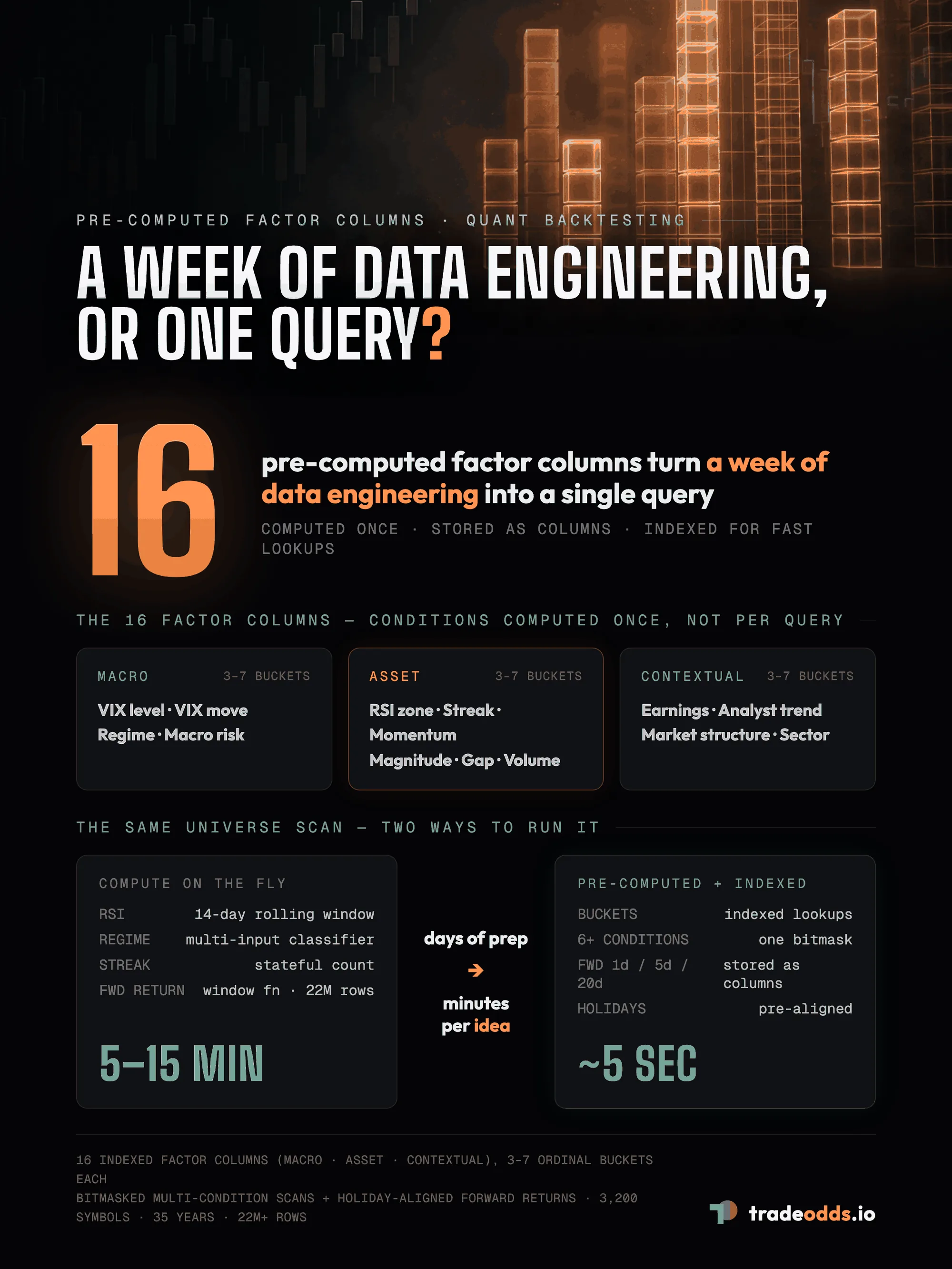
The TradeOdds schema has 16 of these factor columns. They cover:

• Macro: VIX level, VIX move, regime (bull/sideways/bear), macro risk
• Asset: RSI zone, streak, magnitude band, momentum, gap direction, volume
• Contextual: Earnings proximity, analyst trend, market structure, sector strength

Each is bucketed into 3-7 ordinal levels.

Why bucketing instead of raw values

A natural objection: why bucket? Wouldn’t continuous values (raw RSI = 28.4) be more precise than bucketed values (rsi_bucket = -2)?

The answer is two-part:

1. Backtesting at scale needs aggregation, and aggregation needs buckets. “Find every day with RSI between 28 and 30” returns ~100 matches across 35 years. “Find every day with RSI in the oversold bucket (≤ 30)” returns ~3000. The first is too noisy to validate; the second is statistically meaningful. Bucketing is what makes large-N analysis possible.

2. The relationship between conditions and outcomes is rarely sharp. A 28.4 RSI doesn’t behave dramatically differently from a 31.7 RSI. Bucketing acknowledges this and lets the database engine use indexed lookups instead of range scans.

For traders who DO need raw values, the raw columns are still there (rsi_14, vix_level, etc.). Bucket columns are the layer optimized for cross-symbol scans; raw columns are for single-symbol point lookups.

Why this matters for query performance

A query like “find every stock currently in a rare setup and rank by historical edge” — the classic factor scan — has three components:

1. Filter on a combination of conditions.
2. Aggregate historical outcomes per symbol.
3. Rank symbols by the result.

Without pre-computed factor columns, step 1 requires recomputing every condition per row. RSI is a 14-day rolling window. Regime is a classifier over multiple inputs. Streak is a stateful count. Doing this at query time across 22M+ rows takes minutes, not seconds.

With pre-computed factor columns + composite indexes on common combinations, step 1 is a series of index lookups. The same scan runs in single-digit seconds.

The numerical difference: a 16-condition universe scan across 3,200 symbols and 35 years of history runs in ~5 seconds on TradeOdds. The equivalent query against raw OHLCV without pre-computed columns would take 5-15 minutes on the same hardware, assuming you’d built the right indexes in the first place (and you wouldn’t have built them perfectly the first time).

What “bitmasked” adds

Several TradeOdds factor columns are bitmasked. Bitmasking means a single column stores multiple boolean flags in different bit positions, so a single integer can answer “is this row in bucket A AND bucket B AND not in bucket C” with a fast bitwise operation.

For factor scans involving 6+ conditions, this is dramatically faster than checking each condition with a separate comparison. The database engine does one bitwise mask instead of six boolean tests per row.

You don’t write bitwise queries directly — the schema exposes the columns as if they were normal integers. The optimization is invisible. You just benefit.

Pre-computed forward returns

The other half of the factor-column advantage is forward returns as columns. The standard approach to computing a 5-day forward return:

SELECT
  symbol,
  date,
  LEAD(close, 5) OVER (PARTITION BY symbol ORDER BY date) / close - 1 AS fwd_5d
FROM daily_metrics;

This is a window function over 22M rows, partitioned by symbol, ordered by date. It’s slow and brittle (holidays break it; you have to add a trading-calendar join).

TradeOdds pre-computes this:

SELECT symbol, date, fwd_5d_pct
FROM daily_metrics;

fwd_5d_pct is just a column. Holiday-aligned. No window function. Sub-second across 35 years.

The same goes for fwd_1d_pct, fwd_20d_pct, and the open-anchored variants. They’re all columns, all pre-computed.

The practical impact

For a quant trader, this changes the unit of work.

Without pre-computed factors: “I have an idea. Spend Saturday computing the conditions. Spend Sunday joining forward returns and fixing the holiday alignment. Spend Monday actually testing the idea. Spend Tuesday wishing I’d tested a different idea.”

With pre-computed factors: “I have an idea. Open SQL playground. Five minutes later I know whether to bother engineering this further.”

The shift from days to minutes per idea changes how many ideas you can plausibly test. Most quant strategies fail in research; a fast research loop means you find the ones that work without burning your weekend on ones that don’t.

Where to see this in action

In TradeOdds:

• Analyze dashboard (free for 10 lifetime runs, unlimited on Analysis tier+): the UI uses the factor columns under the hood. Toggle a condition and the underlying SQL just adds a bucket = X filter.
• Factor Match (Pro tier+): universe-wide scans across all 3,200+ symbols ranked by historical win rate, made fast by the bucket indexes.
• Direct SQL query (Power User tier and above): write your own queries against daily_metrics with the factor columns directly available.

The full schema is documented at /docs/schema. The factor catalog with bucket definitions is at /docs/factors.

Summary

Pre-computed factor columns are an unsexy infrastructure choice with outsized impact. They turn “spend a week computing what RSI and regime mean” into “filter on rsi_bucket = -2 AND regime_bucket = 1.” They turn “wait three minutes for a universe scan” into “wait three seconds.” For quant traders evaluating data vendors, the presence or absence of this layer is one of the largest practical differences between products.

FAQ

What is a pre-computed factor column?

A derived value — like an RSI zone, market regime, or momentum streak — that has been calculated once, stored as its own column, and indexed for fast lookups. Instead of computing RSI from price every time you query, you filter a column such as rsi_bucket that already holds values from oversold to overbought. The TradeOdds schema has 16 of these factor columns, each bucketed into 3–7 ordinal levels.

Why bucket factors instead of using raw values?

Backtesting at scale needs aggregation, and aggregation needs buckets. Finding every day with RSI between 28 and 30 returns about 100 matches across 35 years — too noisy to validate. Finding every day in the oversold bucket (≤ 30) returns about 3,000 — statistically meaningful. Raw columns like rsi_14 are still available for single-symbol point lookups.

How much faster are pre-computed factor columns?

A 16-condition universe scan across 3,200 symbols and 35 years of history runs in about 5 seconds on TradeOdds using pre-computed columns and composite indexes. The equivalent query against raw OHLCV, recomputing every condition per row across 22M+ rows, takes 5–15 minutes on the same hardware.

What are pre-computed forward returns?

Instead of computing a 5-day forward return with a slow, holiday-breaking window function, TradeOdds stores it as a plain column — fwd_5d_pct — alongside fwd_1d_pct, fwd_20d_pct, and open-anchored variants. They are holiday-aligned and query sub-second across 35 years.

What does bitmasking add?

Several factor columns store multiple boolean flags in different bit positions of a single integer, so a filter involving 6+ conditions runs as one bitwise operation instead of six separate comparisons per row. You query the columns as if they were normal integers — the optimization is invisible.

---

Disclaimer. TradeOdds provides historical analysis for informational purposes only. This is not investment advice. Past performance does not guarantee future results.